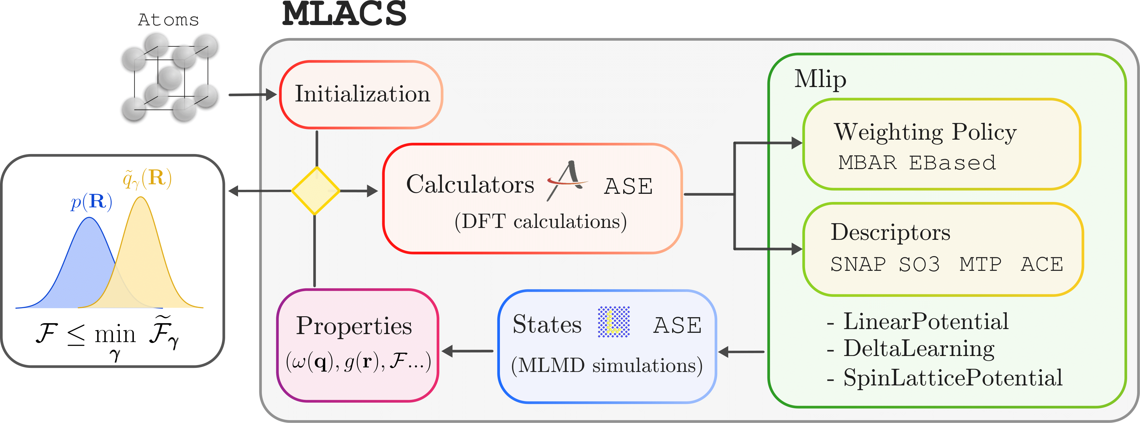
Background

Considering an arbitrary system of \(N_\mathrm{at}\) atoms at a temperature \(T\) inducing a potential \(V(\mathbf{R})\), the classical average of an observable \(O(\mathbf{R})\) is

\[\langle O(\mathbf{R}) \rangle = \int d \mathbf{R} O(\mathbf{R}) p(\mathbf{R}) \approx \sum_n w_n O(\mathbf{R}_n)\]

with \(p(\mathbf{R}) = e^{-\beta V(\mathbf{R})}/\mathcal{Z}\) the Boltzmann weight, \(\mathcal{Z}=\int d\mathbf{R} e^{-\beta V(\mathbf{R})}\) the partition function and \(w_n\) the weight of configuration \(n\) such as \(\sum_n w_n=1\).

In the context of ab initio simulations, obtaining the canonical distribution \(p(\mathbf{R})\) entails costly Ab Initio Molecular Dynamics (AIMD), which can be challenging to perform or even out of reach.

The goal of the Machine-Learning Assisted Canonical Sampling approach is to produce a reduced set of configurations and their associated weight using a Machine-Learning Interatomic Potential (MLIP) in order to approximate the equilibrium canonical distribution and to allow the computation of finite-temperature properties in an ab initio setting.

Theory

Machine-Learning Assisted Canonical Sampling

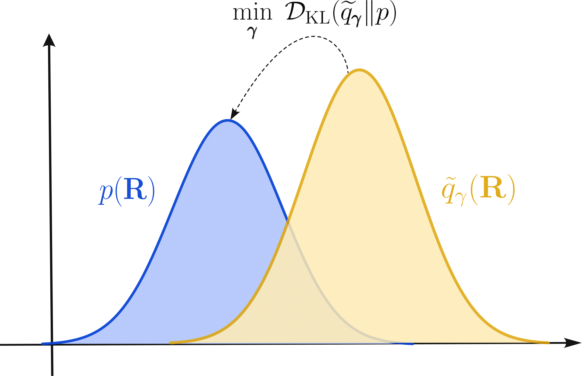
MLACS is built upon the Kullback–Leibler divergence, whose goal is to give a measure of the discrepancy between two distributions \(p(\mathbf{R})\) and \(\widetilde{q}_\gamma(\mathbf{R})\) and is written

\[\mathcal{D}_{KL}(\widetilde{q}_\gamma \Vert p) = \int d\mathbf{R} \widetilde{q}_\gamma(\mathbf{R}) \ln\bigg(\frac{\widetilde{q}_\gamma(\mathbf{R})}{p(\mathbf{R})}\bigg) \geq 0\]

with \(\widetilde{q}_\gamma(\mathbf{R}) = \frac{1}{\widetilde{\mathcal{Z}}} e^{-\beta \widetilde{V}_\gamma(\mathbf{R})}\) the surrogate distribution induced by the MLIP potential \(\widetilde{V}_\gamma(\mathbf{R})\). An important feature of the surrogate potential is its parametrization, indicated by the subscript \(\gamma\), meaning that its shape can be modified by adjusting the parameter \(\boldsymbol{\gamma}\).

With some reorganization, the Kullback–Leibler divergence inequality can be reformulated in term of free energies known as the Gibbs–Bogoliubov inequality

\[\mathcal{F} \leq \widetilde{\mathcal{F}}_\gamma^0 + \langle \mathcal{V}(\mathbf{R}) - \widetilde{\mathcal{V}}_\gamma (\mathbf{R}) \rangle_\gamma\]

where \(\mathcal{F} = -k_BT \ln(\mathcal{Z})\) and \(\widetilde{\mathcal{F}}_\gamma = -k_BT \ln(\widetilde{\mathcal{Z}}_\gamma)\) are the free energies associated with respectively the target and surrogate potentials, and \(\langle \rangle_\gamma\) is the canonical average for the surrogate potential \(\widetilde{V}_\gamma(\mathbf{R})\).

This inequality is at the foundation of the MLACS method. It indicates that by minimizing its right hand side with respect to the parameters \(\boldsymbol{\gamma}\) of the surrogate distribution, one can obtain an optimal approximation for the free energy of the target system. Moreover, due to the relation between the Gibbs–Bogoliubov inequality and the Kullback–Leibler divergence, this optimal free energy approximation also corresponds to an optimal measure of the equilibrium canonical distribution of the target system. Thus, the goal of the MLACS approach is to perform this minimization.

If we assume a linear dependece between the descriptors \(\widetilde{\mathbf{D}}(\mathbf{R})\) and the surrogate potential, the latter writes \(\widetilde{V}_\gamma(\mathbf{R}) = \sum_n \gamma_n \widetilde{D}_n(\mathbf{R})\). This enables a large variety of MLIP, the most known being SNAP, ACE or MTP. By minimizing the Gibbs–Bogoliubov free energy, we obtain the following nontrivial least-squares solution for the optimal parameters

\[\boldsymbol{\gamma} = \langle \widetilde{D}_\gamma(\mathbf{R})^T \widetilde{D}_\gamma(\mathbf{R}) \rangle^{-1} \langle \widetilde{D}_\gamma(\mathbf{R})^T V(\mathbf{R}) \rangle_\gamma\]

with a circular dependency over \(\mathbf{\gamma}\), which can be solved using a self consistent procedure.

Free energy computation

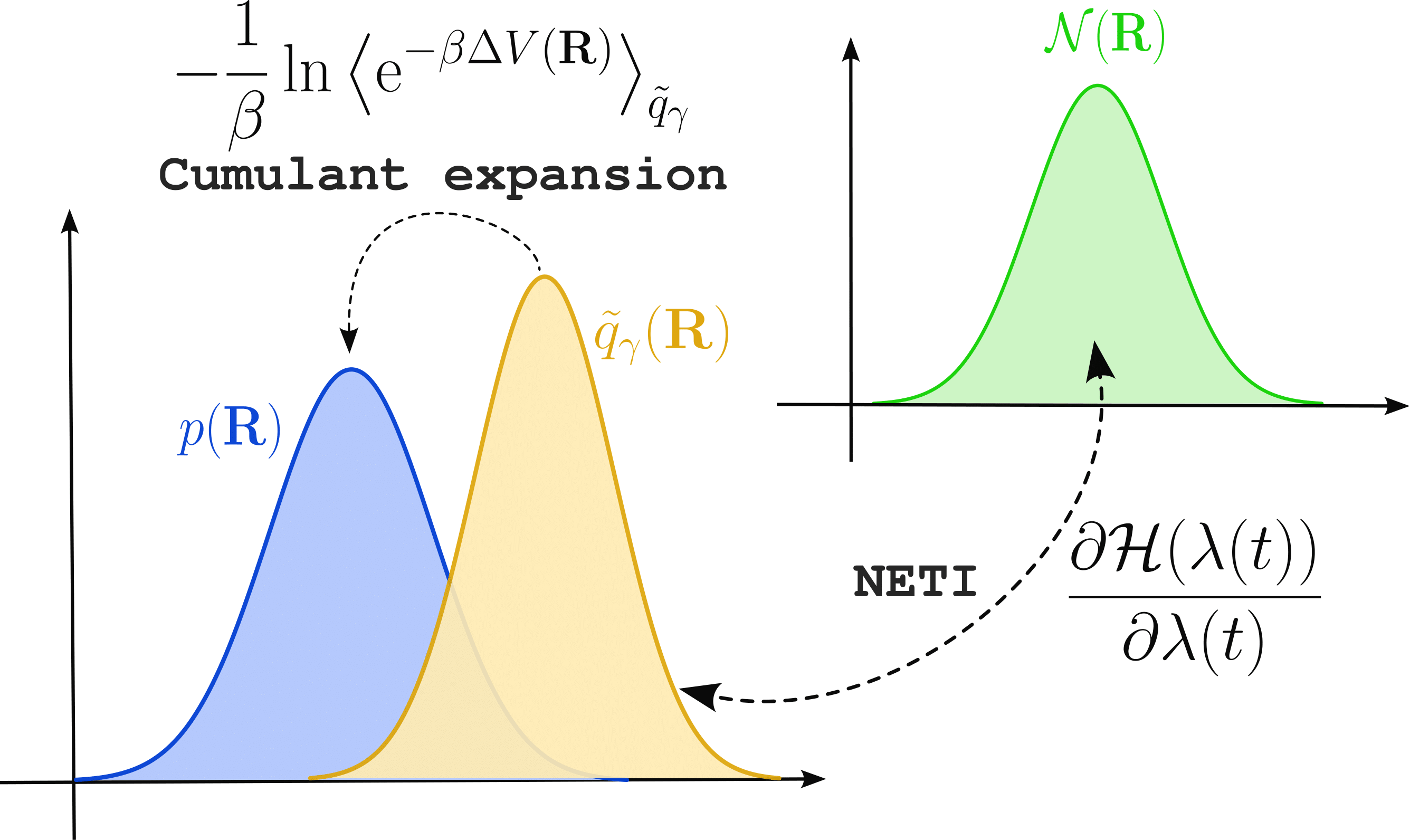
As explained in the previous section, MLACS allows to best approximate the free energy of the system. However, the computation of this approximation necessitates to know the free energy associated with the surrogate model, which generally cannot be obtained analytically. Fortunately, the surrogate free energy \(\widetilde{\mathcal{F}}_\gamma\) can be computed numerically by means of Thermodynamic Integration (TI).

Let us introduce a reference system with a Hamiltonian \(H_\mathrm{ref}\), for which the free energy \(\mathcal{F}_\mathrm{ref}\) is known, and a parametrized Hamiltonian \(H(\lambda) = \lambda \widetilde{H}_\gamma + (1 - \lambda)H_\mathrm{ref}\) with \(\widetilde{H}_\gamma\) the Hamiltonian of the surrogate system. It can be shown that the free energy difference \(\Delta \mathcal{F}_{\mathrm{ref}\rightarrow \gamma} = \widetilde{\mathcal{F}}_\gamma - \mathcal{F}_\mathrm{ref}\) between the reference and surrogate potentials is given by

\[\Delta \mathcal{F}_{\mathrm{ref}\rightarrow \gamma} = \int_0^1 d\lambda \bigg\langle \frac{\partial H(\lambda)}{\partial \lambda} \bigg\rangle_\lambda\]

where \(\langle \rangle_\lambda\) is the canonical average for the Hamiltonian \(H(\lambda)\). Using Jarzynski’s identity, it can be shown that this free energy difference can be computed as an average over various realizations of the irreducible work generated during a non-equilibrium simulation starting from one state and ending in the other. The irreversible work is written as

\[W_{\mathrm{irr}} = \lim_{t_s\rightarrow \infty}\int_0^{t_s} dt \frac{\partial\lambda(t)}{\partial t} \frac{\partial H(\lambda)}{\partial \lambda}\]

Numerically, the effect of noise in the estimation of the free energy difference can be estimated by computing the average between forward and backward simulation between the reference and surrogate Hamiltonian as

\[\Delta \mathcal{F}_{\mathrm{ref}\rightarrow \gamma} = \frac{1}{2} \big( W_{\mathrm{irr}}^{\gamma\rightarrow \mathrm{ref}} - W_{\mathrm{irr}}^{\mathrm{ref}\rightarrow\gamma})\]

Then, the free energy associated with the surrogate model is given by

\[\widetilde{\mathcal{F}}_\gamma = \mathcal{F}_{\mathrm{ref}} + \Delta \mathcal{F}_{\mathrm{ref}\rightarrow \gamma}\]

However, we are interested in the free energy computed at the ab initio level. Despite the great accuracy provided by MLIPs, remaining at this level can generate error that are too large compared to the precision needed in free energy calculation. Thus, it can be important to perform another step consisting in correcting the obtained free energy from the surrogate model to ab initio.

From free energy perturbation theory, we know that the difference \(\Delta \mathcal{F}_{\gamma\rightarrow \mathrm{AI}} = \mathcal{F} - \widetilde{\mathcal{F}}_\gamma\) between ab initio and the surrogate model is written

\[\Delta \mathcal{F}_{\gamma\rightarrow \mathrm{AI}} = \big\langle e^{-\beta \Delta V(\mathbf{R})} \big\rangle_\gamma\]

with \(\Delta V(\mathbf{R}) = V(\mathbf{R}) - \widetilde{V}_\gamma(\mathbf{R})\). This equation can be expanded into cumulants as

\[\Delta \mathcal{F}_{\gamma\rightarrow \mathrm{AI}} = \sum_{n=1}^\infty \frac{(-\beta)^{n-1} \kappa_n}{n!}\]

where \(\kappa_n\) is the \(n\) -th order cumulant of the potential energy difference. Up to second order, the cumulants are given by

\[\begin{split}\kappa_1 =& \langle \Delta V(\mathbf{R}) \rangle_\gamma \\ \kappa_2 =& \langle \Delta V^2(\mathbf{R}) \rangle_\gamma - \langle \Delta V(\mathbf{R}) \rangle_\gamma^2\end{split}\]

Using this cumulant expansion, the free energy difference becomes

\[\Delta \mathcal{F}_{\gamma\rightarrow \mathrm{AI}} \approx \langle \Delta V(\mathbf{R}) \rangle_\gamma + \frac{\beta}{2} \langle \Delta V^2(\mathbf{R}) \rangle_\gamma - \langle \Delta V(\mathbf{R}) \rangle_\gamma^2\]

and the final expression for the free energy at the ab initio level is

\[\mathcal{F} = \mathcal{F}_{\mathrm{ref}} + \Delta \mathcal{F}_{\mathrm{ref}\rightarrow \gamma} + \Delta \mathcal{F}_{\gamma\rightarrow \mathrm{AI}}\]

Implementation