Structural optimization assisted by machine-learning interatomic potentials
In this tutorial, we will show how to perform structural optimization for large structures by using a machine-learning interatomic potential as a surrogate model to reduce the number of potential energy calculation.
Setting up the simulation
As for MLACS, such simulations contains 3 ingredients - The system, which consist in an atomic system and it’s associated potential - A minimization method - A machine-learning interatomic potential
We will start this tutorial by demonstrating the simplest way to set up all these components
Setting up the system
The first component is the actual system to be simulated. In this tutorial, we will simulate vacanies in bulk aluminium with a EMT potential
As input, we can use the bulk function of the ASE package and remove some atoms.
[1]:
from ase.build import bulk
at = bulk("Al", cubic=True).repeat(2)  # This create a 2x2x2 supercell of aluminium

# Let's remove random atoms in the structure
import numpy as np
rng = np.random.default_rng()
for _ in range(3):
    at.pop(rng.integers(0, len(at)))
For the potential, we can use the EMT implementation in ASE
[2]:
from ase.calculators.emt import EMT
calc = EMT()
Setting up the state
The second ingredient for a MLACS simulation is the state to be sampled. Usually, the state is defined by the thermostat/barostat used in the molecular dynamics simulation
We will start by setting up some parameters
[3]:
min_style = 'cg'  # We will use conjugate gradient to minimize
pressure = 0.0  # We will also optimize the cell at 0 pressure
etol = 1e-6  # Energy criterion
ftol = 1e-2  # Forces criterion
stol = 1e-2  # Stress criterion
etol_state = 1e-8  # Energy criterion in the MLIP minimization
ftol_state = 1e-5  # Forces criterion in the MLIP minimization
nsteps = 1000
nsteps_eq = 500
We also have to provide the path to the LAMMPS binary. This can be set up using a bash command
export ASE_LAMMPSRUN_COMMAND=~/.local/bin/lmp
or directly in python as we will do here
[4]:
import os
os.environ["ASE_LAMMPSRUN_COMMAND"] = "lmp"
Now, we can import the state, that will consist here in a LAMMPS optimizer with the parameters defined earlier.
[5]:
from mlacs.state import OptimizeLammpsState
state = OptimizeLammpsState(min_style=min_style,
                            pressure=pressure,
                            etol=etol_state,
                            ftol=ftol_state,
                            nsteps=nsteps,
                            nsteps_eq=nsteps_eq)
Setting up the machine-learning interatomic potential
And the final ingredient is the machine-learning interatomic potential that will drive the molecular dynamics and will be updated from the reference data gathered.
In this example, we will use a SNAP potential with a parameter \(2J_{\mathrm{max}}\) of 8. The setting up of a SNAP potential is done in two steps: * define the descriptor
[6]:
from mlacs.mlip import SnapDescriptor
parameters = {"twojmax": 8}
descriptor = SnapDescriptor(at,
                            parameters=parameters)
Define the model
To improve on the convergence, we will train our potential so that it’s getting better and better as we get closer to the minima. To do this, we will apply some weights for the configurations, in order to give more importance to the configurations close to the minima and less to the one far from it. This can be done by using a WeightingPolicy object which gives more importance to the last configurations added to the dataset. We will use weights given by \(i^{10}\) where i is the index of
the simulation in the dataset (starting at i=1).
[7]:
from mlacs.mlip import LinearPotential, IncreasingWeight
power = 10
energy_coefficient = 1e-5
forces_coefficient = 1
stress_coefficient = 10
weight = IncreasingWeight(power=10,
                          energy_coefficient=energy_coefficient,
                          forces_coefficient=forces_coefficient,
                          stress_coefficient=stress_coefficient)
mlip = LinearPotential(descriptor, weight=weight)
Gathering everything and launching the simulation
Now that everything is set up, we can gather everything into a MlMinimizer object
[8]:
from mlacs import MlMinimizer
dyn = MlMinimizer(at,
                  state,
                  calc,
                  mlip,
                  etol=etol,
                  ftol=ftol,
                  stol=stol)
===============================================================================
            On-the-fly Machine-Learning Assisted Canonical Sampling
            *******************************************************

                      Copyright (C) 2022-2024 MLACS group.
                    MLACS comes with ABSOLUTELY NO WARRANTY.
               This package is distributed under the terms of the
                   GNU General Public License, see LICENSE.md
                    or http://www.gnu.org.copyleft/gpl.txt.

                      MLACS is common project of the CEA,
           Université de Liège, Université du Québec à Trois-Rivières
                 and other collaborators, see CONTRIBUTORS.md.
                  Please read ACKNOWLEDGMENTS.md for suggested
                      acknowledgments of the MLACS effort.
===============================================================================

version 0.0.13

date: 31-10-2024 14:04:45


===============================================================================
                       Recap of the simulation parameters

Recap of the states
*******************
State 1/1 :
Geometry optimization as implemented in LAMMPS
   target pressure: 0.0
   min_style: cg
   energy tolerance: 1e-08
   forces tolerance: 1e-05


Recap of the calculator
***********************
True potential parameters:
Calculator : emt
parameters :


Recap of the MLIP
*****************
Linear potential
Parameters:
-----------
Fit method :            ols

Descriptor used in the potential:
SNAP descriptor
---------------
Elements :
Al
Parameters :
rcut                5.0
chemflag            0
twojmax             8
rfac0               0.99363
rmin0               0.0
switchflag          1
bzeroflag           1
wselfallflag        0
dimension           56


===============================================================================
                            Starting the simulation


Structure optimization assisted by machine-learning
   Energy tolerance: 1e-06 eV/at
   Forces tolerance: 0.01 eV/angs
   Stress tolerance: 0.01 GPa
and launch the simulation for 20 steps
[9]:
dyn.run(20)
===============================================================================
Step 0
Running initial step
There are 1 unique configuration in the states
Computation done, creating trajectories

Computing energy with true potential on training configurations

===============================================================================
Step 1

Equilibration step for state 1, configurations 1 for this state

Training new MLIP

Number of configurations for training: 2
Number of atomic environments for training: 58

Using Increasing weighting
Weighted RMSE Energy    0.0001 eV/at
Weighted MAE Energy     0.0001 eV/at
Weighted RMSE Forces    0.0011 eV/angs
Weighted MAE Forces     0.0007 eV/angs
Weighted RMSE Stress    0.0001 GPa
Weighted MAE Stress     0.0000 GPa

Running MLMD
 -> Starting from first atomic configuration
State 1/1 has been launched
Computing energy with the True potential
Energy difference :  2.619 eV/at
Maximum absolute force : 0.0094487 eV/angs
Maximum stress tensor difference : 0.16906 GPa

===============================================================================
Step 2

Equilibration step for state 1, configurations 2 for this state

Training new MLIP

Number of configurations for training: 3
Number of atomic environments for training: 87

Using Increasing weighting
Weighted RMSE Energy    0.0004 eV/at
Weighted MAE Energy     0.0004 eV/at
Weighted RMSE Forces    0.0001 eV/angs
Weighted MAE Forces     0.0000 eV/angs
Weighted RMSE Stress    0.0001 GPa
Weighted MAE Stress     0.0000 GPa

Running MLMD
 -> Starting from first atomic configuration
State 1/1 has been launched
Computing energy with the True potential
Energy difference : 5.2068e-05 eV/at
Maximum absolute force : 0.0028278 eV/angs
Maximum stress tensor difference : 0.15035 GPa

===============================================================================
Step 3

Equilibration step for state 1, configurations 3 for this state

Training new MLIP

Number of configurations for training: 4
Number of atomic environments for training: 116

Using Increasing weighting
Weighted RMSE Energy    0.0000 eV/at
Weighted MAE Energy     0.0000 eV/at
Weighted RMSE Forces    0.0001 eV/angs
Weighted MAE Forces     0.0000 eV/angs
Weighted RMSE Stress    0.0001 GPa
Weighted MAE Stress     0.0000 GPa

Running MLMD
 -> Starting from first atomic configuration
State 1/1 has been launched
Computing energy with the True potential
Energy difference : 0.0002691 eV/at
Maximum absolute force : 0.002296 eV/angs
Maximum stress tensor difference : 0.073075 GPa

===============================================================================
Step 4

Equilibration step for state 1, configurations 4 for this state

Training new MLIP

Number of configurations for training: 5
Number of atomic environments for training: 145

Using Increasing weighting
Weighted RMSE Energy    0.0000 eV/at
Weighted MAE Energy     0.0000 eV/at
Weighted RMSE Forces    0.0001 eV/angs
Weighted MAE Forces     0.0000 eV/angs
Weighted RMSE Stress    0.0001 GPa
Weighted MAE Stress     0.0000 GPa

Running MLMD
 -> Starting from first atomic configuration
State 1/1 has been launched
Computing energy with the True potential
Energy difference : 3.9882e-06 eV/at
Maximum absolute force : 0.00048199 eV/angs
Maximum stress tensor difference : 0.0019739 GPa

===============================================================================
Step 5

Equilibration step for state 1, configurations 5 for this state

Training new MLIP

Number of configurations for training: 6
Number of atomic environments for training: 174

Using Increasing weighting
Weighted RMSE Energy    0.0000 eV/at
Weighted MAE Energy     0.0000 eV/at
Weighted RMSE Forces    0.0000 eV/angs
Weighted MAE Forces     0.0000 eV/angs
Weighted RMSE Stress    0.0001 GPa
Weighted MAE Stress     0.0000 GPa

Running MLMD
 -> Starting from first atomic configuration
State 1/1 has been launched
Computing energy with the True potential
Energy difference : 2.2213e-06 eV/at
Maximum absolute force : 0.0012512 eV/angs
Maximum stress tensor difference : 0.0012699 GPa

===============================================================================
Step 6

Equilibration step for state 1, configurations 6 for this state

Training new MLIP

Number of configurations for training: 7
Number of atomic environments for training: 203

Using Increasing weighting
Weighted RMSE Energy    0.0000 eV/at
Weighted MAE Energy     0.0000 eV/at
Weighted RMSE Forces    0.0000 eV/angs
Weighted MAE Forces     0.0000 eV/angs
Weighted RMSE Stress    0.0001 GPa
Weighted MAE Stress     0.0000 GPa

Running MLMD
 -> Starting from first atomic configuration
State 1/1 has been launched
Computing energy with the True potential
Energy difference : 2.8182e-06 eV/at
Maximum absolute force : 0.00018546 eV/angs
Maximum stress tensor difference : 0.0013483 GPa

===============================================================================
Step 7

Equilibration step for state 1, configurations 7 for this state

Training new MLIP

Number of configurations for training: 8
Number of atomic environments for training: 232

Using Increasing weighting
Weighted RMSE Energy    0.0000 eV/at
Weighted MAE Energy     0.0000 eV/at
Weighted RMSE Forces    0.0000 eV/angs
Weighted MAE Forces     0.0000 eV/angs
Weighted RMSE Stress    0.0001 GPa
Weighted MAE Stress     0.0000 GPa

Running MLMD
 -> Starting from first atomic configuration
State 1/1 has been launched
Computing energy with the True potential
Energy difference : 2.1733e-06 eV/at
Maximum absolute force : 0.00051055 eV/angs
Maximum stress tensor difference : 0.0010896 GPa

===============================================================================
Step 8

Equilibration step for state 1, configurations 8 for this state

Training new MLIP

Number of configurations for training: 9
Number of atomic environments for training: 261

Using Increasing weighting
Weighted RMSE Energy    0.0000 eV/at
Weighted MAE Energy     0.0000 eV/at
Weighted RMSE Forces    0.0000 eV/angs
Weighted MAE Forces     0.0000 eV/angs
Weighted RMSE Stress    0.0000 GPa
Weighted MAE Stress     0.0000 GPa

Running MLMD
 -> Starting from first atomic configuration
State 1/1 has been launched
Computing energy with the True potential
Energy difference : 6.3877e-07 eV/at
Maximum absolute force : 0.00044712 eV/angs
Maximum stress tensor difference : 0.0010119 GPa


===============================================================================
              Convergence criteria reached, stoping the simulation
===============================================================================

===============================================================================
                      Copyright (C) 2022-2024 MLACS group.
                    MLACS comes with ABSOLUTELY NO WARRANTY.
               This package is distributed under the terms of the
                   GNU General Public License, see LICENSE.md
                    or http://www.gnu.org.copyleft/gpl.txt.

                      MLACS is common project of the CEA,
           Université de Liège, Université du Québec à Trois-Rivières
                 and other collaborators, see CONTRIBUTORS.md.
===============================================================================

===============================================================================
                  Suggested acknowledgments of the MLACS usage
                  ********************************************

The MLACS theory and algorithm
A. Castellano, F. Bottin, J. Bouchet, A. Levitt, G. Stoltz
Phys. Rev. B 106, L161110 (2022)

The MLACS package
A. Castellano, R. Béjaud, P. Richard, O. Nadeau, G. Geneste,
G. Antonius, J. Bouchet, A. Levitt, G. Stoltz, F. Bottin
(To be submitted (2024))
===============================================================================
And that’s it !
The simulations, computed with the reference potential, can be found in the Trajectory.traj file
[10]:
from ase.io import read
confs = read("Trajectory.traj", index=":")
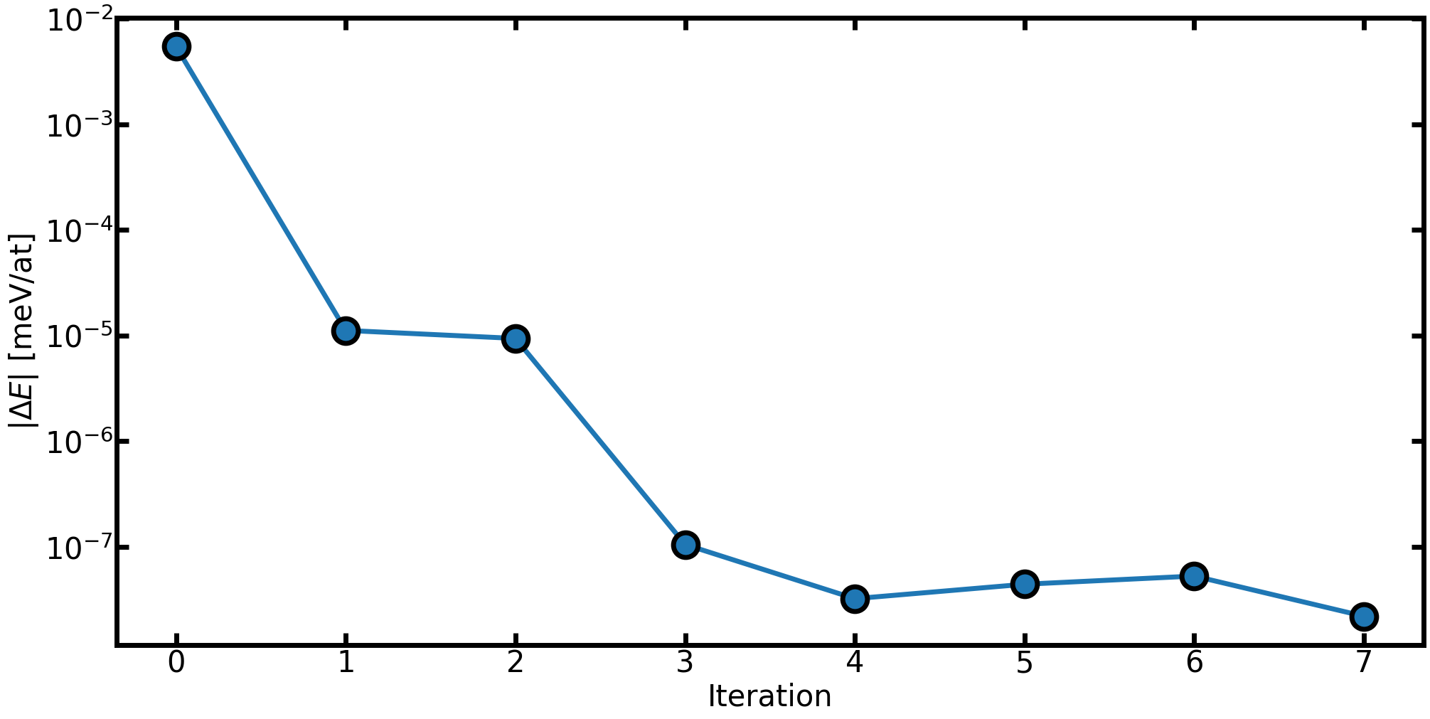
And we can plot for example the energy along the trajectory to observe that we reach the minimum
[13]:
import numpy as np
import matplotlib.pyplot as plt
from mlacs.utilities.plots import init_rcParams

x = np.arange(len(confs))
energies = np.array([a.get_potential_energy() / len(a) for a in confs])

fig = plt.figure(figsize=(20, 10), constrained_layout=True)
init_rcParams()
ax0 = fig.add_subplot()
ax0.set_xlabel("Iteration")
ax0.set_ylabel(r"$|\Delta E|$ [meV/at]")  # Potential energy difference
Delta_E = energies - energies[-1]
ax0.plot(x[:-1], np.abs(Delta_E[:-1]), marker="o")  # Do not plot last iteration (zero by construction)
ax0.set_yscale("log")
plt.show()
[ ]: