Training a Moment Tensor Potential model

In this tutorial, we will see how to train a machine-learning interatomic potential with the MTP model

As for the SNAP example, we need to export the path to the LAMMPS binary with

export ASE_LAMMPSRUN_COMMAND=/path/to/lmp_serial

or directly inside the python script as we will do here

import os

os.environ["ASE_LAMMPSRUN_COMMAND"] = "lmp"

Once this is done, we can open the dataset using the io module of ASE

from ase.io import read

configurations = read("../Data/Silicon.traj", index=":")

This dataset correspond to 20 configurations of crystaline Silicon in a 2x2x2 supercell with displacements

print(configurations[0])
print(len(configurations))

Atoms(symbols='Si64', pbc=True, cell=[10.873553019744607, 10.873553019744607, 10.873553019744607], momenta=..., calculator=SinglePointCalculator(...))
20

For the MTP potential, the descriptor and model are handled directly with the the MLIP package. For this kind of potential, we only need to import the MomentTensorPotential

from mlacs.mlip import MomentTensorPotential

To initialize the descriptor, we need to give it some parameters.

mtp_params = dict(max_dist=4.5,
                  min_dist=1.5,
                  level=4)
fit_params = dict(max_iter=50,
                  bfgs_conv_tol=1e-3)

We also need to define the path to the mtp binary

mlpbin = "mlp"

We can now initalize our model with this descriptor

mlip = MomentTensorPotential(configurations[0],
                             mlpbin,
                             mtp_parameters=mtp_params,
                             fit_parameters=fit_params)

We can check the parameters of our MLIP

print(repr(mlip))

Moment Tensor Potential
Parameters:
-----------
Descriptor:
-----------
level :                 4
radial basis function : RBChebyshev
Radial basis size :     8
Minimum distance :      1.5
Cutoff :                4.5

To train the model, we need now to add the configurations to the training set.

This is done with the update_matrices function of the potential, that takes either an ASE atoms object or a list of atoms.

mlip.update_matrices(configurations)

The model can now be trained using the train_mlip function

msg = mlip.train_mlip()
print(msg)

mlp train /home/bejaudr/software/Mlacs/otf_mlacs/tutorials/Mlip/MomentTensorPotential/MTP/initpot.mtp /home/bejaudr/software/Mlacs/otf_mlacs/tutorials/Mlip/MomentTensorPotential/MTP/train.cfg --trained-pot-name=/home/bejaudr/software/Mlacs/otf_mlacs/tutorials/Mlip/MomentTensorPotential/MTP/pot.mtp --update-mindist --init-params=random --max-iter=50 --bfgs-conv-tol=0.001 --scale-by-force=0 --energy-weight=1.0 --force-weight=1.0 --stress-weight=1.0 --weighting=vibrations

---------------------------------------------------------------------------
KeyboardInterrupt                         Traceback (most recent call last)
/tmp/ipykernel_18460/2692604443.py in <module>
----> 1 msg = mlip.train_mlip()
      2 print(msg)

~/software/Mlacs/otf_mlacs/mlacs/mlip/mtp_model.py in train_mlip(self, mlip_subfolder)
    193         self._write_input(subfolder=subfolder)
    194         self._write_mtpfile(subfolder=subfolder)
--> 195         self._run_mlp(subfolder=subfolder)
    196
    197         # Symlink new MTP in the main folder

~/software/Mlacs/otf_mlacs/mlacs/mlip/mtp_model.py in _run_mlp(self, subfolder)
    306                              stderr=PIPE,
    307                              stdout=fd,
--> 308                              cwd=subfolder)
    309         if mlp_handle.returncode != 0:
    310             msg = "mlp stopped with the exit code \n" + \

/usr/lib/python3.7/subprocess.py in run(input, capture_output, timeout, check, *popenargs, **kwargs)
    488     with Popen(*popenargs, **kwargs) as process:
    489         try:
--> 490             stdout, stderr = process.communicate(input, timeout=timeout)
    491         except TimeoutExpired as exc:
    492             process.kill()

/usr/lib/python3.7/subprocess.py in communicate(self, input, timeout)
    952                 self.stdout.close()
    953             elif self.stderr:
--> 954                 stderr = self.stderr.read()
    955                 self.stderr.close()
    956             self.wait()

KeyboardInterrupt:

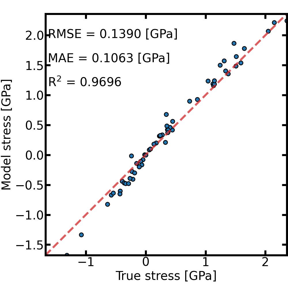
To check the accuracy of our MLIP, we can use the command line mlacs correlation to plot the correlation between DFT data and MLIP prediction.

%%sh
mlacs correlation MLIP-Energy_comparison.dat --size 10 --datatype energy --save EnergyCorrelation.jpeg --noshow
mlacs correlation MLIP-Forces_comparison.dat --size 10 --datatype forces --save ForcesCorrelation.jpeg --noshow
mlacs correlation MLIP-Stress_comparison.dat --size 10 --datatype stress --save StressCorrelation.jpeg --noshow

And that’s it ! The model is ready to be used and can be found in the Snap directory. The pair_style and pair_coeff needed to use it in LAMMPS can be obtained from the mlip object

print(mlip.pair_style)
print(mlip.pair_coeff)

Of course, in real applications the parameters and the size of the dataset will need to be different to obtain an accurate model.