Training a Spectral Neighbor Analysis Potential

In this tutorial, we will see how to train a machine-learning interatomic potential with the SNAP model

As a fist step, we will need to indicate where is the binary to run LAMMPS. This can be done with a bash command to run before running the script

export ASE_LAMMPSRUN_COMMAND=/path/to/lmp_serial

Or directly inside the python script as we will do here

import os

os.environ["ASE_LAMMPSRUN_COMMAND"] = "lmp"

Once this is done, we can open the dataset using the io module of ASE

from ase.io import read

configurations = read("../Data/Silicon.traj", index=":")

This dataset correspond to 20 configurations of crystaline Silicon in a 2x2x2 supercell with displacements

print(configurations[0])
print(len(configurations))

Atoms(symbols='Si64', pbc=True, cell=[10.873553019744607, 10.873553019744607, 10.873553019744607], momenta=..., calculator=SinglePointCalculator(...))
20

To train our MLIP, we need a descriptor and a model. In this example, we will use a simple linear model with the SO(4) descriptor, which correspond to the Spectral Neighbor Analysis Potential. These can be imported from the mlip module

from mlacs.mlip import LinearPotential, SnapDescriptor

To initialize the descriptor, we need to give it some parameters.

snap_params = dict(twojmax=5)
desc = SnapDescriptor(configurations[0], 4.5, snap_params)

We can now initalize our model with this descriptor

mlip = LinearPotential(desc)

We can check the parameters of our MLIP

print(repr(mlip))

Linear potential
Parameters:
-----------
Fit method :            ols

Descriptor used in the potential:
SNAP descriptor
---------------
Elements :
Si
Parameters :
rcut                4.5
chemflag            0
twojmax             5
rfac0               0.99363
rmin0               0.0
switchflag          1
bzeroflag           1
wselfallflag        0
dimension           21

To train the model, we need now to add the configurations to the training set.

This is done with the update_matrices function of the potential, that takes either an ASE atoms object or a list of atoms.

mlip.update_matrices(configurations)

The model can now be trained using the train_mlip function

msg = mlip.train_mlip()
print(msg)

Number of configurations for training: 20
Number of atomic environments for training: 1280

Using Uniform weighting
Weighted RMSE Energy    0.0016 eV/at
Weighted MAE Energy     0.0013 eV/at
Weighted RMSE Forces    0.0749 eV/angs
Weighted MAE Forces     0.0532 eV/angs
Weighted RMSE Stress    0.1607 GPa
Weighted MAE Stress     0.1144 GPa

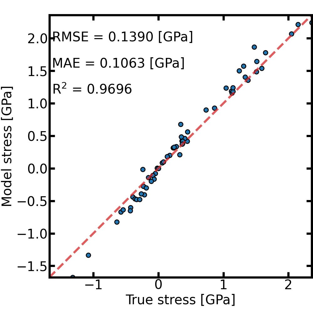
To check the accuracy of our MLIP, we can use the command line mlacs correlation to plot the correlation between DFT data and MLIP prediction.

%%sh
mlacs correlation MLIP-Energy_comparison.dat --size 10 --datatype energy --save EnergyCorrelation.jpeg --noshow
mlacs correlation MLIP-Forces_comparison.dat --size 10 --datatype forces --save ForcesCorrelation.jpeg --noshow
mlacs correlation MLIP-Stress_comparison.dat --size 10 --datatype stress --save StressCorrelation.jpeg --noshow

And that’s it ! The model is ready to be used and can be found in the Snap directory. The pair_style and pair_coeff needed to use it in LAMMPS can be obtained from the mlip object

print(mlip.pair_style)
print(mlip.pair_coeff)

snap
['* * /home/duvalc/mlacs/tutorials/Mlip/Snap/MLIP/SNAP.model  /home/duvalc/mlacs/tutorials/Mlip/Snap/MLIP/SNAP.descriptor Si']

Of course, in real applications the parameters and the size of the dataset will need to be different to obtain an accurate model.